

Brilliant in Excel – Have you ever stared at an Excel spreadsheet, feeling overwhelmed and clueless about where to start? You’re not alone. Excel is a powerful tool, but without the right functions, it can be a daunting maze. Fear not, dear readers! In this article, we’re going to demystify the world of Excel functions. We’ll explore five essential functions that will not only simplify your tasks but also boost your productivity to new heights. So, grab your virtual pens and let’s dive in!

Introduction to Brilliant in Excel Functions
Picture this: you have a massive dataset, and you need to perform various calculations on it. This is where Excel functions come to your rescue. These functions are predefined formulas that make your number-crunching tasks a breeze. Instead of manually calculating values, you can let Excel do the heavy lifting for you.
SUM: Your Number Crunching Ally – Brilliant in Excel
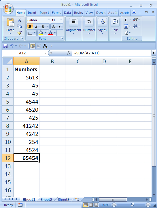
Let’s start with the basics. The SUM function is your trusty sidekick when it comes to adding up numbers in a range. Whether you’re tallying monthly expenses or analyzing sales figures, SUM effortlessly calculates the total. Just select the cells you want to add, enter the SUM function, and voila! Your total magically appears.
Example: Suppose you have a column of numbers from A2 to A10 (A2:A10) representing monthly sales. To find the total sales, you would enter the following formula in an empty cell:
=SUM(A2:A10)
. Excel would add up all the numbers in the specified range and display the result in the cell with the formula.
VLOOKUP: Finding the Needle in the Haystack – Brilliant in Excel
Ever struggled to find specific information in a sea of data? Enter VLOOKUP. This function acts like a digital detective, helping you locate precise details within your spreadsheet. Whether you’re managing inventories or organizing contact lists, VLOOKUP searches for a value in the first column of your table and retrieves data from a specified column. It’s like finding a needle in a haystack without breaking a sweat.
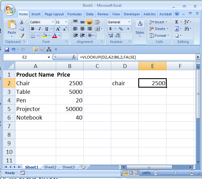
Example: Let’s say you have a table with product names in column A and their corresponding prices in column B. You want to find the price of a specific product, say “Chair.” The formula would look like this:
=VLOOKUP("Chair", A2:B100, 2, FALSE)
. Excel would search for “WidgetX” in column A, and when found, return the value from the adjacent cell in column B.
IF: Logic Made Easy – Brilliant in Excel
Logic in Excel? Absolutely! The IF function allows you to introduce conditions in your spreadsheet. Want to categorize expenses as high, medium, or low? IF can do that. Need to grade student scores based on predefined criteria? IF has your back. It’s like having a built-in decision maker, ensuring your data is sorted and organized according to your rules.
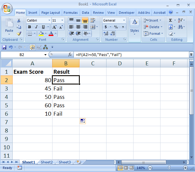
Example: Suppose you have a column of exam scores from A2 to A10. You want to categorize the scores as “Pass” if they are greater than or equal to 50 and “Fail” otherwise. The formula would be:
=IF(A2>=50, "Pass", "Fail")
. Excel would evaluate each score and display “Pass” or “Fail” accordingly.
INDEX-MATCH: The Dynamic Duo – Brilliant in Excel
While VLOOKUP is handy, it has limitations. That’s where the INDEX-MATCH combo steps in. Imagine a tool that not only finds your data but also adapts to changes in your spreadsheet. INDEX-MATCH does just that. By combining these functions, you can search for a specific value across rows and columns, making your search dynamic and foolproof.
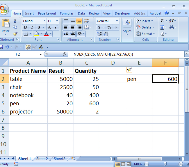
Example: Let’s say you have a table with products in column A, their prices in column B, and quantities in column C. You want to find the quantity of a specific product, say “GadgetY.” The formula would be:
=INDEX(C2:C100, MATCH("GadgetY", A2:A100, 0))
. INDEX-MATCH would search for “GadgetY” in column A and return the corresponding quantity from column C.
CONCATENATE: Merging Cells Simplified
Tired of copying and pasting data into a single cell? CONCATENATE is here to save you time and effort. This function allows you to merge text from multiple cells into one. Whether you’re creating personalized greetings or generating email addresses, CONCATENATE ensures your data is neatly combined, making your spreadsheet look polished and professional.
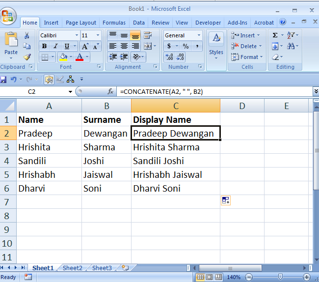
Example: Suppose you have first names in column A (A2:A10) and last names in column B (B2:B10). You want to create a list of full names in column C. The formula would look like this:
=CONCATENATE(A2, " ", B2)
. Excel would merge the first name, a space, and the last name, creating a full name in column C.
Conclusion: Mastering Excel, One Function at a Time
Congratulations, you’ve embarked on a journey to Excel mastery! By mastering these fundamental functions, you’ve unlocked the door to a world of efficient data management and analysis. Remember, Excel is not just about numbers; it’s about empowering you to make informed decisions, faster and smarter.
FAQs: Your Burning Questions Answered
Q1: What is the SUM function, and how is it useful in Excel?
The SUM function in Excel is used to add up numbers in a range of cells. It’s incredibly useful when you need to calculate totals, such as adding sales figures or tallying expenses.
Q2: When should I use VLOOKUP in my spreadsheets?
VLOOKUP is ideal when you want to search for a value in the first column of your table and retrieve data from a specified column. It’s perfect for tasks like managing inventories, looking up prices, or organizing contact lists.
Q3: How does the IF function enhance Excel’s functionality?
The IF function introduces logic into your spreadsheets. It allows you to set conditions based on which certain actions are performed. For instance, you can categorize data, assign grades, or sort information based on specific criteria.
Q4: What makes INDEX-MATCH a superior choice over VLOOKUP?
INDEX-MATCH is superior to VLOOKUP because it’s more flexible. VLOOKUP can only search for values from left to right, but INDEX-MATCH can search both horizontally and vertically. It adapts to changes in your data layout, ensuring accurate results even when your spreadsheet evolves.
Q5: Can you provide an example of CONCATENATE in action?
Certainly! Let’s say you have columns for first names and last names. You can use CONCATENATE to merge these into a single column, creating full names. The formula would look like this:
=CONCATENATE(A2, " ", B2)
where A2 is the first name, B2 is the last name, and the space between the quotes ensures a space between the names.